Is het niet zo dat:
correlatie = 0.95 => (0.95)^2 = 0.9025 van de variatie is 'verklaard'? Dus dan niet overeenkomt voor 95% maar voor 90%.
Correlatie van 0.6 wordt dan 36%.
Wouter
Een terechte opmerking. Voor zover ik de documentatie kon nagaan wordt door jou genoemde gekwadrateerde correlatiecoefficient gebruikt, gek alleen dat de legenda dit niet zo weergeeft.
Van de bronsite van de grafieken: ,, Each model verified against its own analysis. The anomaly correlation score measures the ability of a numerical forecast to represent general weather patterns of high pressure ridges and low pressure troughs, and the locations and strengths of fronts and major storms. It has a maximum value of 1.0 (a perfect depiction of the location of major weather systems), while a score above 0.6 is still considered useful by forecasters. It is universally accepted as a standard score by international weather modeling centers and the World Meteorological Organization.''
Lijkt mij een beetje sterk dat 0,6² = 36% nog als waardevol zou worden beschouwt, 60% lijkt me realistischer, vandaar dat ik ook uitging van R².
Edit: nu ik dit schrijf en dingen opzoek, kom ik de definitie tegen die ze hanteren:
,,Measures of forecast and analysis variance are taken as root-mean-squared amplitudes A and F:
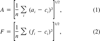
,,. where ai is the analysis value, fi the forecast value, and ci the climatological value at point i. The number of points in the summation (over space or time) is n. The two “basic” integrated statistics used are the root-mean-squared error E and the anomaly correlation R, defined as''
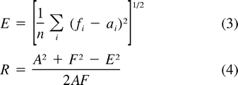
Ik kan niet goed inschatten in hoeverre deze definitie afwijkt van de gebruikelijke ACC (anomaly correlation coefficient) (zie bijv. hier voor de ECMWF definitie) en of deze al gekwadrateerd is en dus het percentage verklaarde variantie weergeeft.
Als je opmerking terecht blijkt dat zal ik mijn verhaal uiteraard aanpassen, dan is de grens voor bruikbaarheid dus bij 36% verklaarde variantie.
Gr. Ben